Characterizing the Local Instability of Orbits in Broad Parameter Spaces

by Juan C. Vallejo and Miguel A.F. Sanjuán

Nonlinear dynamics and chaos are present in many fields of astrodynamics. Computation of distributions of finite time Lyapunov exponents provides valuable information on the local stability of the orbits. When dealing with huge sets of model parameter values, Grid-based techniques make such explorations faster than common techniques.

After the three-body problem was demonstrated to be non-integrable in 1887, the fully analytical approach to orbital dynamics problems was replaced by a time-series approach and the search for limited sets of orbits of particular interest. In the last century, the numerical approach has gained in relevance with the increase in computational facilities. Methods derived from chaos theory, born from a topological approach to this problem, have enjoyed a similar rate of progress. Today, nonlinear dynamics techniques are quite useful in real problems where chaos is present and both stable and unstable orbits must be considered.

A basic method for understanding the dynamics of a given potential is to search several types of existing invariants. Fixed points are first located and characterized, and the associated periodic orbits are then explored. These are considered to be the basis of the observed dynamics, as Poincaré noted in the case of the three-body problem. Their stability properties give an insight into their neighbourhood, since stable orbits are generally surrounded by quasi-periodic ones, and unstable periodic orbits by chaotic ones. This apparently simple scheme is not always straightforward to follow, as the complexity of high-order orbits rapidly confuses the situation. One useful and widely used approach is to compute the invariant tori and invariant manifolds. Another (complementary) approach is to compute orbital stability indicators, such as the Lyapunov exponents, the Rotation Index, the Smaller Alignment Index (SALI) or the Mean Exponential Growth Factor of Nearby Orbits (MEGNO).

Figure 1: Local Lyapunov exponent distributions can characterize a given orbit. In this figure, a quasi-periodic orbit distribution shows the peaks associated with the Poincaré cross-section tori islands.

The ordinary Lyapunov exponents describe the evolution in time of the distance between two nearly initial conditions, and are quite simple to compute independently on the number of degrees of freedom of the problem. A main disadvantage is their slow convergence towards the final value as they are defined as a limit when time tends to infinity. In practice, all calculations are performed numerically, finite times are used, and only approximated values are obtained. But these finite time integrations provide information on the transient dynamics that may occur during relevant time scales, and this may in itself be of interest.

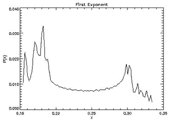
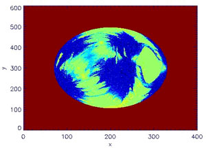
When computed during finite intervals, the Lyapunov exponents are named finite time Lyapunov exponents. When the time interval is reduced to an arbitrary small quantity, they are known as local Lyapunov exponents. These values capture the very local orbital behaviour of the dynamics, and their distribution characterizes it. Our work in the Nonlinear Dynamics and Chaos Group at the Universidad Rey Juan Carlos in Madrid, is focused on analysing certain potentials through the usage of these finite time indicators.

We wanted to explore a huge set of initial conditions and model parameter values, using standard computational resources rather than cutting-edge computers. Grid-based technologies were therefore used, meaning that the required computational runs were divided into small sets to be executed in different available computational resources. These computers reside virtually in the same organization/project, but physically can be in different places and organizations. Grid projects are based on sets of computers that use a Grid Engine such as SGE, Condor or MPI, receive the computational requests, process them, and return the results using a common protocol (usually Globus as de facto protocol). The user, through the Globus layer, or typically through the usage of a friendlier layer such as Condor-G, GridWay or Nimrod, can send the requests, monitor them, or transfer the computations to selected sets of computers.

Figure 2: When plotting Lyapunov exponents for given initial conditions, fractal structures are created and destroyed depending on the model parameter values, showing how stable and unstable regions are mixed in a complex way.

The key driver for our project at URJC is to reuse existing algorithms and computational tools in a Grid environment. Each computational run is based on the integration of one initial condition with a well-known Runge-Kutta(-Fehlberg) integrator scheme. The local Lyapunov exponent distribution is calculated and saved. We repeat this for several conditions and parameters. Using GridWay, the Grid interface has been easy to implement. A set of shell scripts feed the integrator with the proper set of initial conditions, parameter values and data identifiers. These scripts also include the GridWay commands for submitting the jobs and receiving the results. GridWay executes them in the remote machines in a user-transparent way. This wrapper strategy can be used for facing different problems and potentials with only minor modifications.

Links:
http://www.escet.urjc.es/~fisica/
http://www.gridway.org

Please contact:
Juan C. Vallejo, Universidad Rey Juan Carlos, Madrid, Spain
Tel: +34 91 8131366
E-mail: juancarlos.vallejourjc.es